6 Maps

To build a flexible system for mapping cruise data, we have the following functions:

Publishable maps

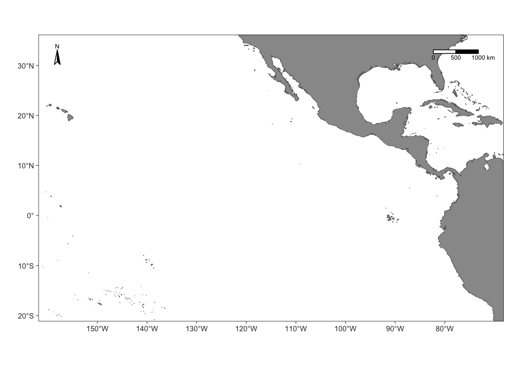
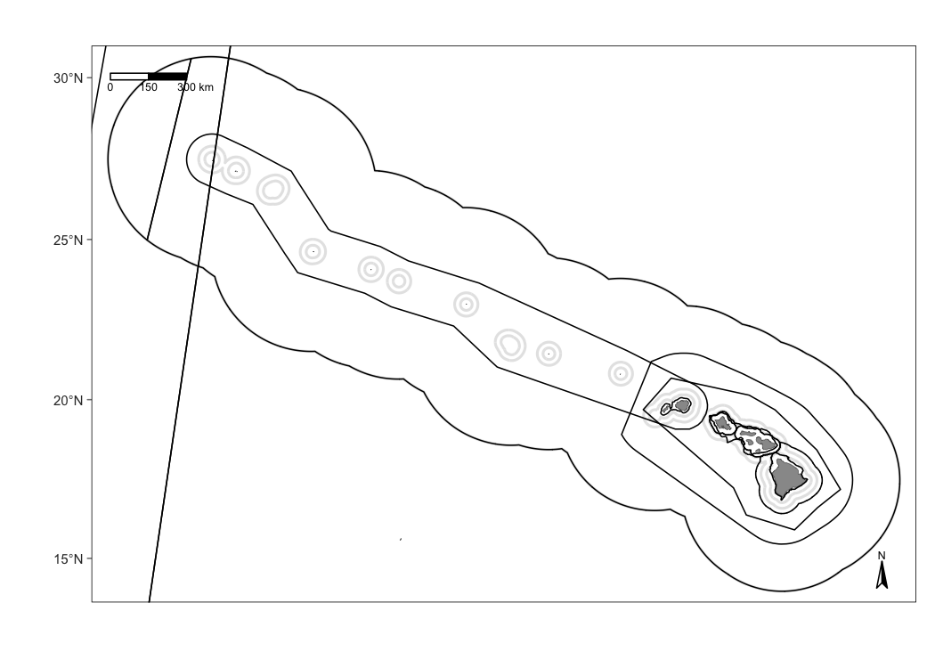
Base maps

Begin with a basic map of the waters surrounding the Hawaiian archipelago, including EEZ borders:

m <- map_base(region='cnp')

# Show map
m

We also have a base map for the California Current …

m <- map_base(region='ccs')

# Show map
m

And the ETP:

m <- map_base(region='etp')

# Show map
m

Add strata

Add your research strata to your map:

m <- map_base(region='cnp')

m1 <- map_strata(m,
                cruz_1720$settings, 
                region='cnp')

# Show map
m1

Add survey tracks

To demonstrate how to map data, we will use survey data from 2017 and 2020 within the WHICEAS study area:

# Load the cruz object we made in the "Processing" chapter
load('whiceas_cruz.RData')

# Filter
cruz_1720 <- 
  filter_cruz(cruz,
              analysis_only = TRUE,
              years = c(2017, 2020),
              regions = 'WHICEAS')

Here is the function that maps effort:

m1 <- map_effort(m, cruz_1720)

# Show map
m1

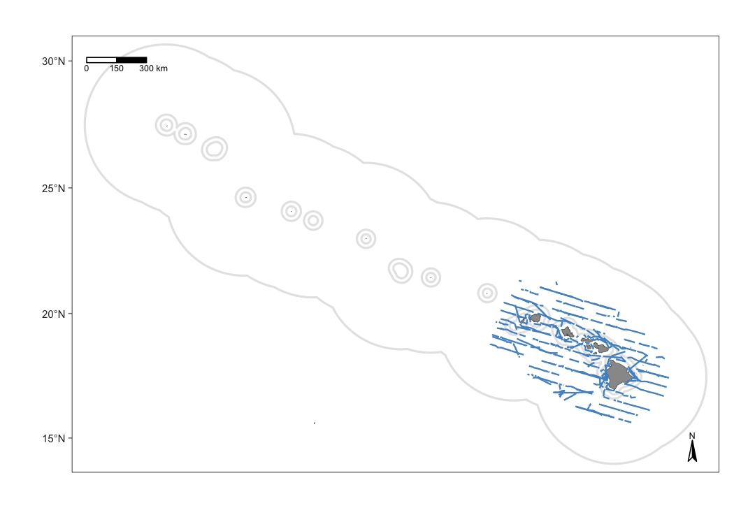
The defaults of map_effort() assume, for simplicity, that you want to see the segments to be included in density estimation for the first cohort specified in your settings. You can adjust this and other defaults using the function arguments.

Customizing effort

Inputs

This map changes survey track thickness and color.

m1 <- map_effort(m, 
                cruz_1720,
                effort_color='firebrick',
                effort_stroke=2.5,
                effort_linetype=1,)

# Show map
m1

Color-code conditions

Your second customization option is to add format variables to the segments slot of the cohort of interest in the cruz object. This gives you full control of line color, thickness, and line-type according to whatever specifications you wish to set, e.g., color-coding by effort type or Beaufort sea state.

This is possible because the function map_effort() looks for the variables col (line color), lwd (line thickness or stroke), and lty (line type) in the columns of cruz$segments. If these columns exist, the values therein will be used instead of the function defaults.

For example, color-code by Beaufort scale:

# Save copy of segments to modify
cruzi <- cruz_1720
segments <- cruzi$cohorts$all$segments

# Add column `col`: color code by BFT sea state
bft_colors <- c('steelblue4','steelblue2','cadetblue1','grey')
segments$col <- bft_colors[4]
segments$col[ segments$avgBft <= 7 ] <- bft_colors[3] # bft 5 +
segments$col[ segments$avgBft <= 4 ] <- bft_colors[2] # bft 3 - 4
segments$col[ segments$avgBft <= 2 ] <- bft_colors[1] # bft 0 -2

# Update sub_segments slot in `cruz` object
cruzi$cohorts$all$segments <- segments

# Update map 
m_custom2 <- map_effort(m, cruzi)

# Add legend using native functions from mapping package `tmap`
m_custom2 <- 
  m_custom2 + 
  tmap::tm_add_legend('line', 
                        col = bft_colors,
                        lwd = 3,
                        labels = c(' 0 - 2', 
                                   ' 3 - 4', 
                                   ' 5 +', 
                                   ' no data'),
                         title="Beaufort sea state") +
  tmap::tm_layout(legend.position=c('left','bottom'))

# Show map
m_custom2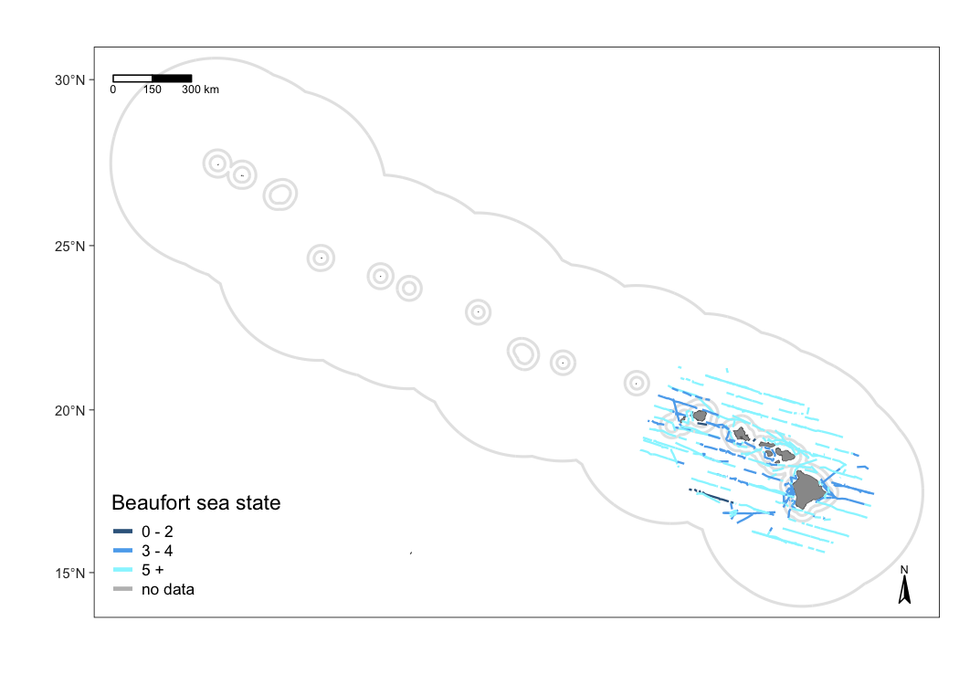

Add sightings

Use the function map_sightings() to add sightings to your map:

m1 <- map_sightings(m, cruz_1720)

# Show map
m1

Customizing sightings

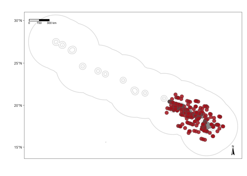
To demonstrate some of the customization options, consider this map that shows sightings of false killer whales with custom dot color, shape, and size:

m1 <- map_sightings(m,
                    cruz_1720,
                    include_species = '033',
                    color_base = 'purple',
                    shape_base = 18,
                    size_base = 1)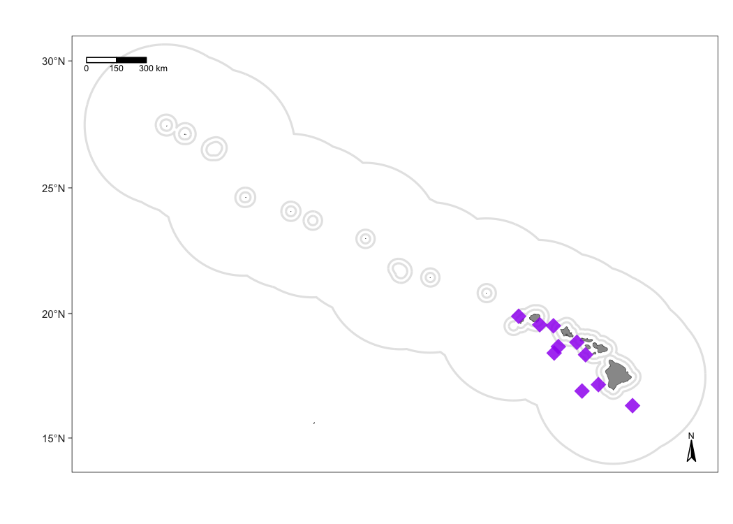

Next is a map of humpback whales and sperm whales, color-coded by species and shape-coded by whether or not the sighting will be included in the analysis:

m1 <- map_sightings(m, 
                   cruz_1720,
                   include_species = c('076','046'),
                   color_code = TRUE,
                   shape_code = TRUE)

# Show map
m1

Overview

Here is an overview of the steps needed to map strata, survey tracks, and sightings all together:

m <- map_base('cnp') 
m <- map_strata(m, cruz_1720$settings)
m <- map_effort(m, cruz_1720)
m <- map_sightings(m, cruz_1720, size_base=.4)
m 

Interactive maps

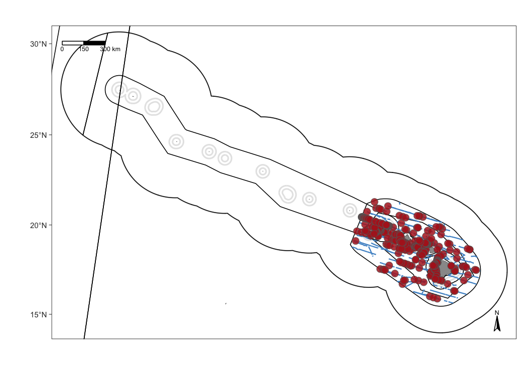
LTabundR also has an interactive map function, which maps survey data using the leaflet package.

 map_cruz(cruz_1720,
          cohort=1,
          eez_show=FALSE,
          strata_show=FALSE,
          effort_show=TRUE,
          effort_resolution=1,
          sightings_show=TRUE,
          sightings_color = 'firebrick',
          verbose=FALSE)

Note that you can also click on sightings and tracklines to see their details. Refer to the documentation for this function (?map_cruz) to see all the options available for stylizing these maps.

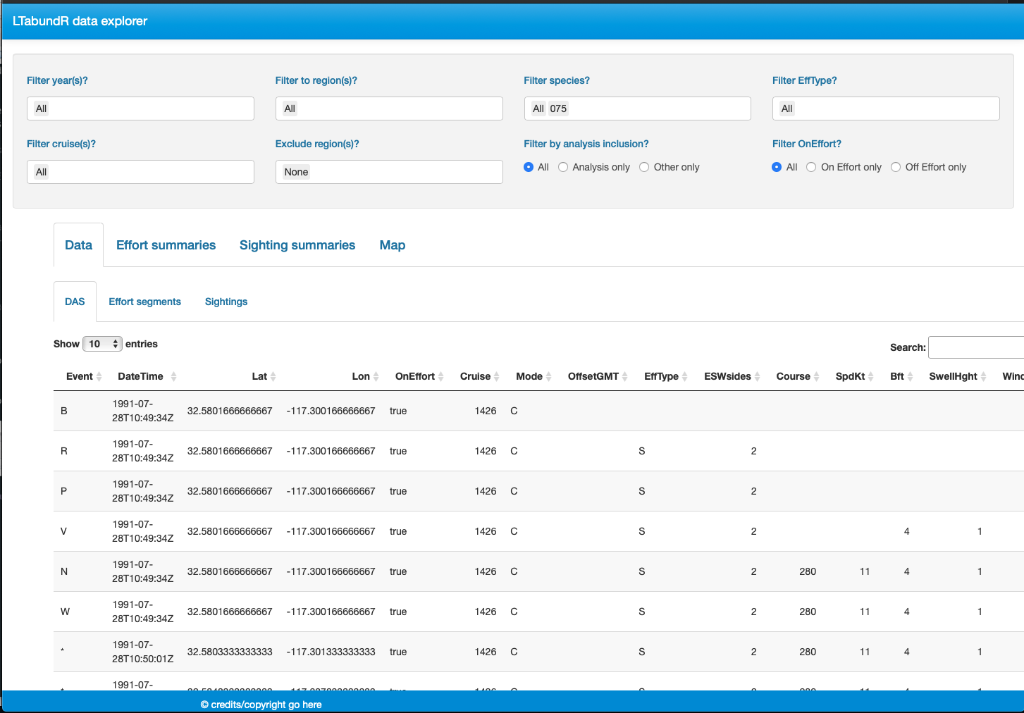
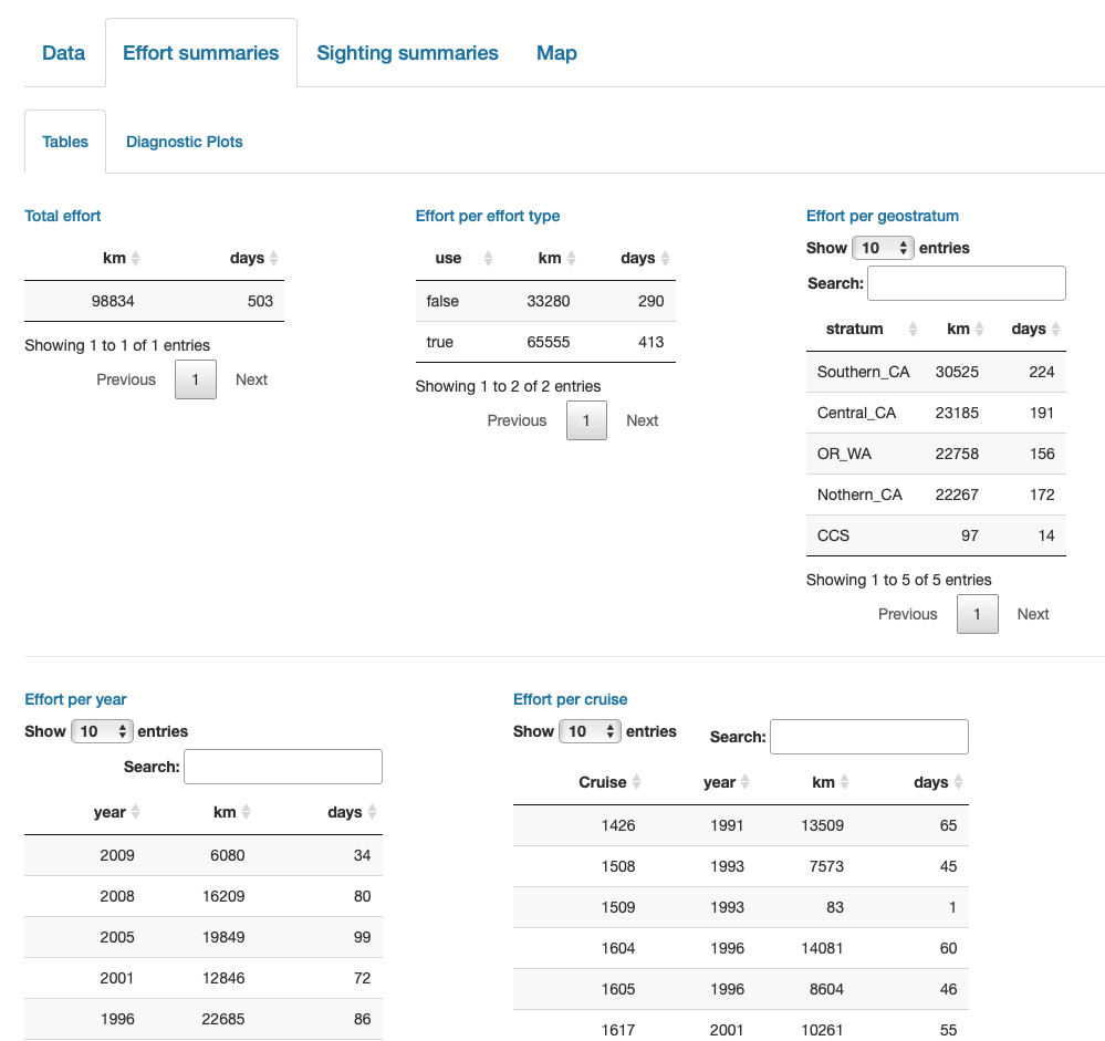
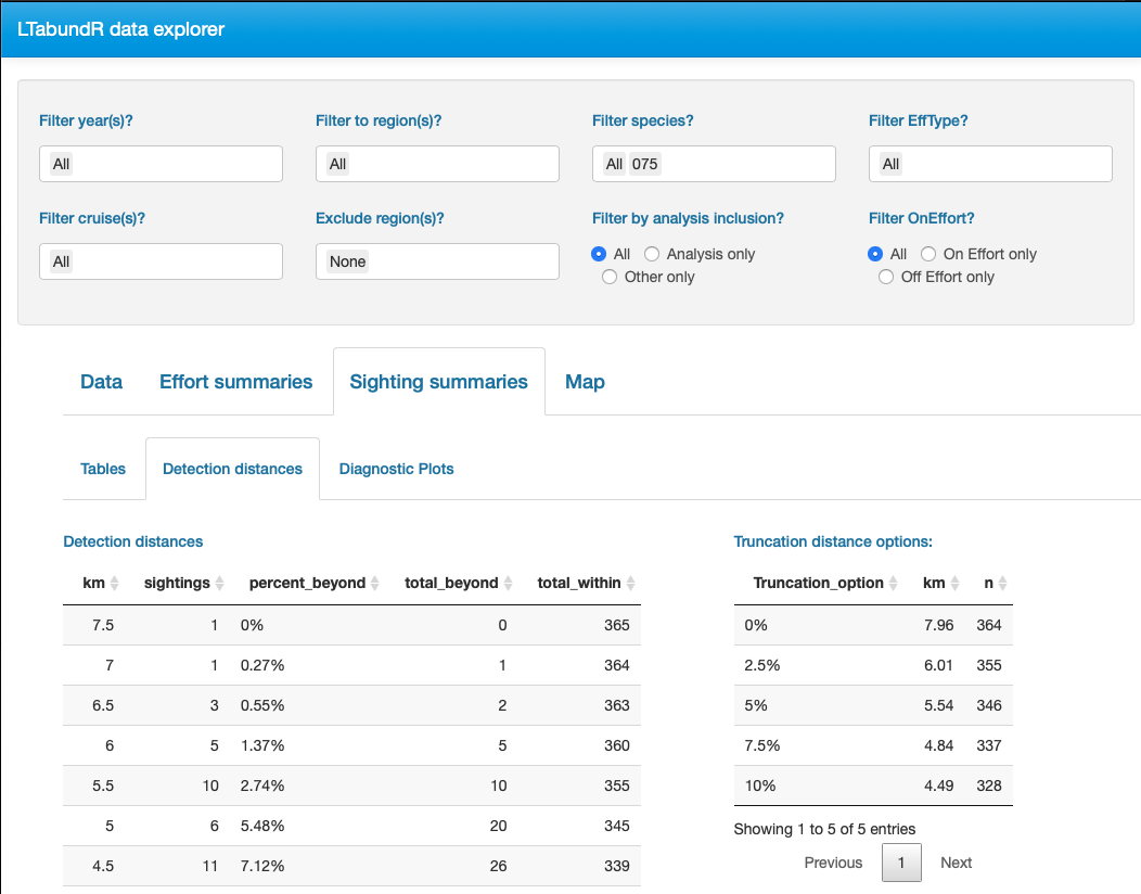
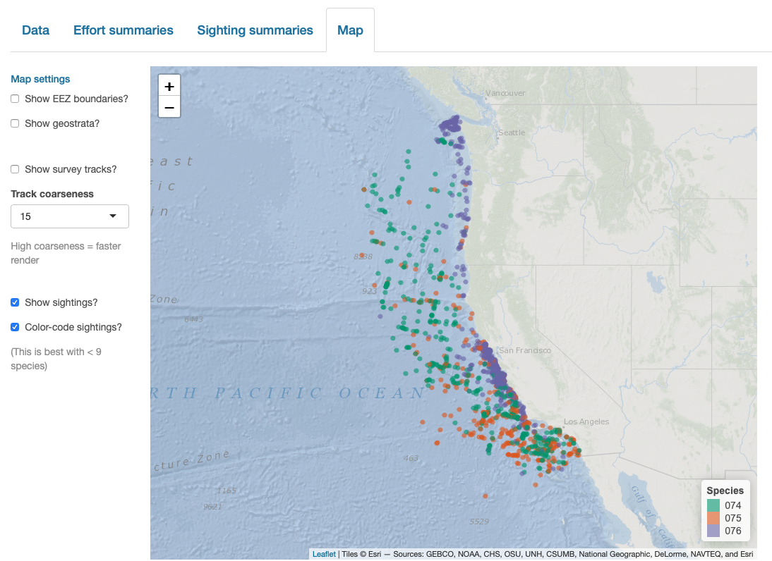
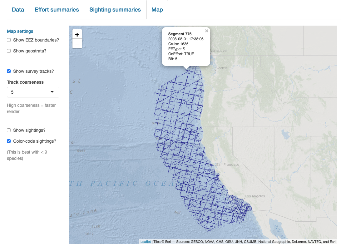
Interactive dashboard

Finally, note that LTabundR comes with an interactive data explorer app (a Shiny app) for filtering survey data according to effort scenario and species code, toggling map_cruz() settings, and reviewing summary tables of effort and sightings (including inspection of truncation distances).

cruz_explorer(cruz)

Screenshots from this app: